Fourier Transform Notes
These are just notes I put on this website so that I will be able to remeber the content and be able to review it easly for later exams. This is not meant to go into full detail about the Fourier Transform, so stuff like derivations and proofs will not be included b/c deriving this stuff requires a lot more research than I'd like to do.
Fourier Transform
Fourier Transform
Inverse Fourier Transform
One of the main purposes of the Fourier Transform is to point out the dominant frequencies of a waveform. This can easily be seen with the FT of a regular sine or cosine wave.
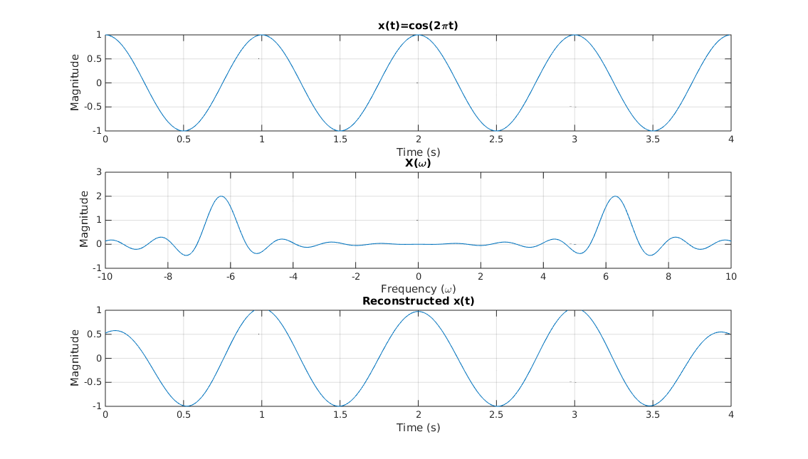
The FT of a cosine wave is the dirac delta functions at \(+ω_0\) and \(-ω_0\). This makes sense since the only frequency in a regular cosine wave is \(ω_0\). The reason for the peak at \(-ω_0\) is because the FT of real waves are always symmetrical across the initial phase shift. In this case, φ = 0, so the FT of \(cos(2πt)\) will be symmetrical across the y-axis.
For the example above, the FT is not an exact dirac function since I am only integrating over a finite set of data rather than an infinite set from t = -∞ to +∞. If I had more data points, the peaks would stand out more. Similarly, the reconstruction of x(t) from X(ω) is not exactly the same as the original x(t) because of the finite amount of data points I am integrating over in the frequency domain. For the continuous FT, the FT converts continuous data in the time domain to continous data in the frequency domain.
Discrete Time Fourier Transform
Discrete Time Fourier Transform of x[n]
Inverse Fourier Transform of X(ω)
In the real world though, data is not necessarily continuous. In the example used to generate x(t), I just found x(t) at very small increments of t to replicate continuous data. Really, I just took discrete values of x(t) sampled every Ts seconds. The DTFT allows us to essentially take the Fourier Transform of discrete/sampled data, though the spectrum is different in the frequency domain than the continuous FT.
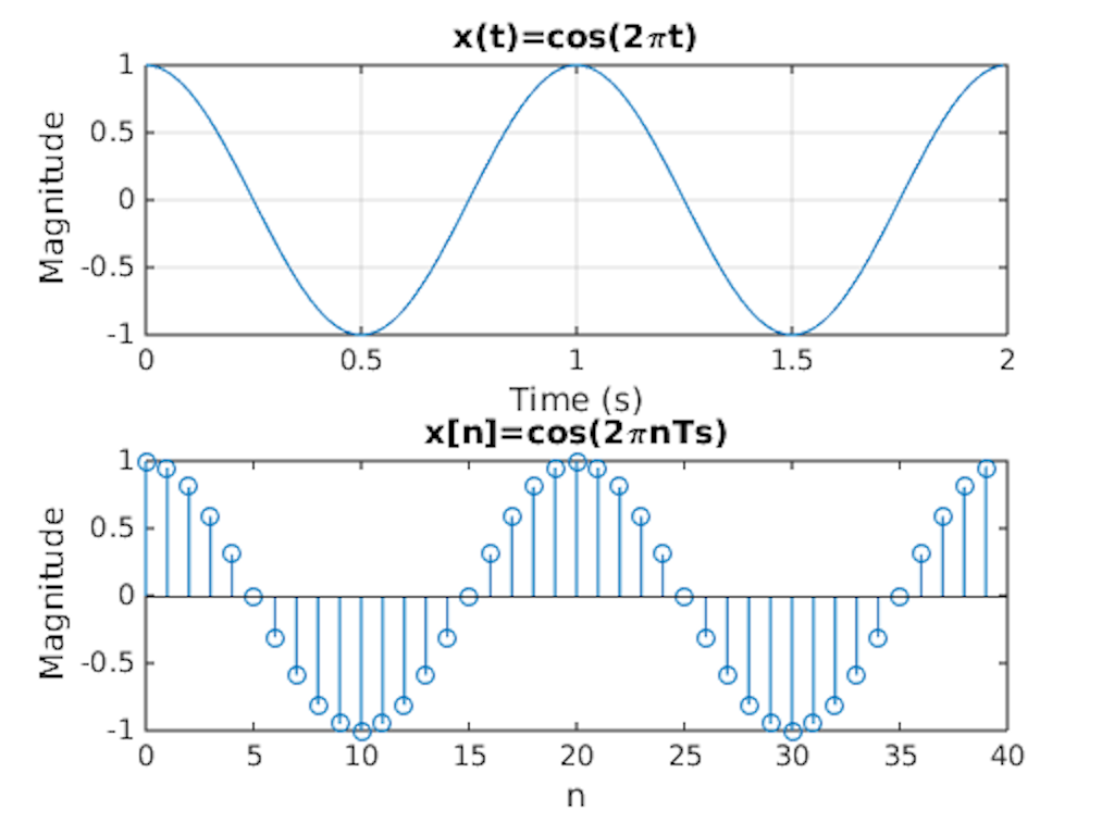
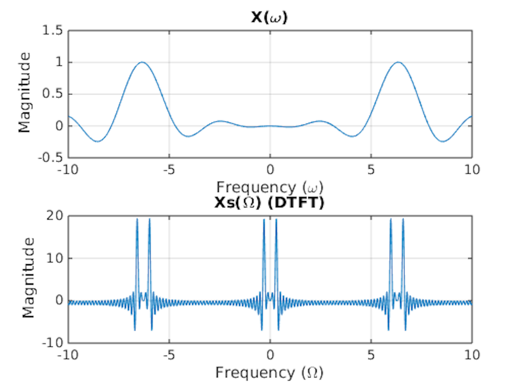
In the example above, I take the FT of a continuous cosine wave and the DTFT of the cosine wave sampled every Ts seconds. In this case, Ts = 0.05 s and my sampling frequency (fs) = 20 Hz. The FT of x(t) returns X(ω), which should be two dirac delta functions at positive and negative \(ω_0\). The DTFT of x[n], however, returns Xs(Ω). This spectrum is different from that of the FT in that:
- The DTFT is in terms of Ω while the FT is in terms of ω, where \(X_s(Ω)\) = \(X_s(ωTs)\). (A similar example of this notation is how x[n] = x(nTs).) Though both have the same units (rad/s), the scale of the DTFT is smaller than that of the FT by a factor of the sampling frequency (fs = 1/Ts).
- The DTFT repeats every 2π. This is because the DTFT is the sum of various FTs at frequencies that are 2π apart from each other.
- The DTFT transforms discrete data from the time domain to continuous data in the frequency domain while the FT transforms continuous data in the time domain to continuous data in the frequency domain.
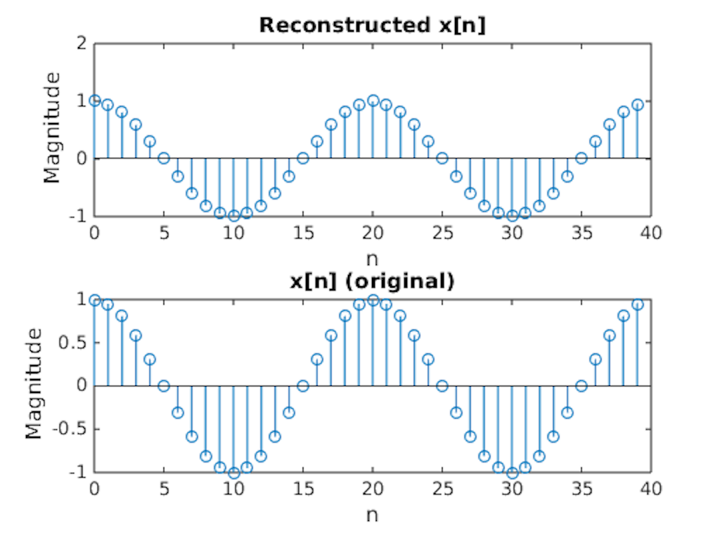
Like the IFT, the original discrete signal can also be reconstructed from its DTFT. Theoretically, the continuous signal could be constructed from the discrete signal, though this would require an infinitely large sampling frequency to replicate an infinitesimally small dt.
